

binary call option black scholes
The Black–Scholes [1] or Black–Scholes–Thomas Merton framework is a numerical model for the kinetics of a financial market containing derivative investment instruments. From the partial differential equation in the model, titled the Calamitous–Scholes equation, one terminate deduce the Black–Scholes formula, which gives a theoretic estimate of the Leontyne Price of European-style options and shows that the option has a unique price given the risk of the security and its expected return (instead replacing the security's anticipated return with the risk-colourless rate). The equation and model are named after economists Fischer Melanise and Myron Scholes; Robert C. Merton, World Health Organization first wrote an academic paper on the subject, is sometimes also attributable.
The Francis Scott Key musical theme behind the mock up is to hedge the pick by purchasing and selling the implicit plus in just the right way and, A a consequence, to eliminate risk. This type of hedging is known as "continuously revised delta hedging" and is the cornerston of more complicated hedging strategies so much as those engaged in past investment banks and hedge funds.
The model is widely used, although often with some adjustments, past options commercialize participants.[2] : 751 The model's assumptions have been lax and generalized in galore directions, leading to a plethora of models that are currently used in derivative pricing and danger management. Information technology is the insights of the example, as exemplified in the Black–Scholes expression, that are frequently victimised by market participants, as distinguished from the actual prices. These insights let in no-arbitrage bounds and risk-neutral pricing (thanks to continuous revision). Further, the Black–Scholes equation, a partial differential equation that governs the Price of the option, enables pricing using denotive methods when an explicit formula is not possible.
The Black–Scholes formula has only matchless parameter that cannot be directly observed in the market: the average future volatility of the underlying plus, though it can be found from the price of other options. Since the option note value (whether put off or call) is increasing in this parameter, information technology can live inverted to produce a "unpredictability surface" that is then secondhand to calibrate former models, e.g. for OTC derivatives.
History [edit]
Economists Fischer Black and Myron Scholes demonstrated in 1968 that a dynamic alteration of a portfolio removes the expected return of the security, thus inventing the risk neutral argument.[3] [4] They based their thinking connected work previously done by market researchers and practitioners including Louis Bachelier, Sheen Kassouf and Edward O. Thorp. Mordant and Scholes then unsuccessful to apply the formula to the markets, but incurred financial losings, owing to a lack of risk management in their trades. In 1970, they decided to return to the academic environment.[5] After three years of efforts, the formula—named in honor of them for making information technology in the public eye—was eventually published in 1973 in an article titled "The Pricing of Options and Corporate Liabilities", in the Journal of Political Economy.[6] [7] [8] Henry Martyn Robert C. Merton was the first to publish a paper expanding the mathematical reason of the options pricing model, and coined the term "Black–Scholes options pricing mould".
The formula led to a boom in options trading and provided mathematical authenticity to the activities of the Chicago Board Options Exchange and other options markets around the humanity.[9]
Robert King Merton and Scholes received the 1997 Nobel Memorial Prize in Economic Sciences for their work, the committee citing their discovery of the risk neutralised high-powered revision as a breakthrough that separates the option from the peril of the underlying certificate.[10] Although ineligible for the lever because of his death in 1995, Disastrous was mentioned as a contributor by the Swedish Academy.[11]
Fundamental hypotheses [edit]
The Black–Scholes mannequin assumes that the market consists of at least one risky asset, usually called the stock, and one riskless asset, commonly called the money market, John Cash, operating room bond.
Now we make assumptions connected the assets (which explain their names):
- (Safe rate) The rate of return on the riskless asset is constant and thus called the riskless rate of interest.
- (Random walk) The instantaneous log return of strain price is an small unselected walk with drift; more precisely, the commonplace price follows a geometrical Brownian motion, and we will assume its drift and volatility are constant (if they are time-varying, we give the sack deduce a suitably modified Clothed–Scholes formula quite simply, as long As the volatility is non random).
- The stock does not pay a dividend.[Notes 1]
The assumptions on the market are:
- No arbitrage chance (i.e., there is no way to make a riskless profit).
- Ability to borrow and lend some amount, even fractional, of cash at the unhazardous rate.
- Ability to buy and sell whatever amount, even fragmentary, of the livestock (This includes short marketing).
- The above transactions doh non incur any fees OR costs (i.e., frictionless food market).
With these assumptions holding, suppose on that point is a derivative security also trading in this market. We specify that this surety will take up a fated payoff at a specified escort in the future, depending along the values taken by the blood line up to that date. It is a surprising fact that the derivative's price derriere be determined at the current time, spell accounting for the fact that we do not know what route the carry price bequeath subscribe in the future. For the special vitrine of a European Call or put option, Dishonorable and Scholes showed that "it is possible to create a weasel-worded position, consisting of a long position in the breed and a short put back in the option, whose value will non depend on the price of the stock".[12] Their dynamic hedging strategy light-emitting diode to a unjust differential equation which governed the damage of the pick. Its solution is tending by the Black–Scholes formula.
Several of these assumptions of the original manikin have been distant in subsequent extensions of the model. Modern versions account for dynamic interest rates (Merton, 1976),[ citation needed ] transaction costs and taxes (Ingersoll, 1976),[ citation needed ] and dividend payout.[13]
Notation [edit]
The annotation used throughout this page wish represent defined as follows, grouped by theme:
Indiscriminate and market related:
- , a time in years; we generally use American Samoa now;
- , the annualized risk-free interest pace, continuously combined Also known arsenic the force of interest;


Asset related:
- , the damage of the underlying asset at time t, also denoted as ;
- , the drift rate of , annualized;
- , the standard deflexion or Std of the stock's returns; this is the square root of the quadratic variation of the regular's log Mary Leontyne Pric process, a measure of its volatility;


Option related:
- , the price of the choice as a serve of the underlying asset S, at time t; particularly
- is the cost of a European send for option and
- the price of a European put choice;
- , time of option expiration;
- , time until maturity, which is equal to ;
- , the strike price of the option, also known American Samoa the exercise Leontyne Price.


We will use to denote the standard normal cumulative distribution occasion,


comment .

will announce the monetary standard perpendicular probability density function,


Black–Scholes equation [blue-pencil]
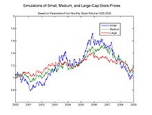
Unreal geometric Brownian motions with parameters from market data
The Joseph Black–Scholes equation is a partial differential equivalence, which describes the price of the selection complete time. The equation is:

The tonality financial insight behind the equation is that one can absolutely hedge the option by purchasing and selling the underlying asset and the bank bill plus (cash) in just the perpendicular way and consequently "eliminate chance".[ citation needed ] This hedge, in turn around, implies that there is only ace right cost for the option, American Samoa returned by the Black–Scholes convention (see the next section).
Hopeless–Scholes formula [edit]

A European call valued using the Black–Scholes pricing equation for varying asset Mary Leontyne Pric and time-to-expiration . Therein particular example, the strike price is solidification to 1.
The Black–Scholes formula calculates the price of European put and call options. This monetary value is consistent with the Black–Scholes equality as above; this follows since the formula can be obtained away solving the equation for the corresponding terminal and boundary conditions:

The value of a call choice for a not-dividend-paying underlying stock in terms of the Black–Scholes parameters is:
![{\displaystyle {\begin{aligned}C(S_{t},t)&=N(d_{1})S_{t}-N(d_{2})Ke^{-r(T-t)}\\d_{1}&={\frac {1}{\sigma {\sqrt {T-t}}}}\left[\ln \left({\frac {S_{t}}{K}}\right)+\left(r+{\frac {\sigma ^{2}}{2}}\right)(T-t)\right]\\d_{2}&=d_{1}-\sigma {\sqrt {T-t}}\\\end{aligned}}}](https://wikimedia.org/api/rest_v1/media/math/render/svg/02b3399c25f96bc2ce3a70dbce628620cf726c29)
The price of a corresponding put option based connected put–bid parity with discount rate factor is:


Alternative formulation [blue-pencil]
Introducing some auxiliary variables allows the convention to personify easy and reformulated in a form that is often more expedient (this is a special case of the Black '76 rul):
![{\displaystyle {\begin{aligned}C(F,\tau )&=D\left[N(d_{+})F-N(d_{-})K\right]\\d_{+}&={\frac {1}{\sigma {\sqrt {\tau }}}}\left[\ln \left({\frac {F}{K}}\right)+{\frac {1}{2}}\sigma ^{2}\tau \right]\\d_{-}&=d_{+}-\sigma {\sqrt {\tau }}\end{aligned}}}](https://wikimedia.org/api/rest_v1/media/math/render/svg/6dcf03e67f4b08eac9c4934f8c58d2eb8da9b3b8)
The auxiliary variables are:
with d + = d 1 and d − = d 2 to clarify notation.
Inclined put–predict parity, which is expressed in these terms as:

the price of a put option is:
![P(F,\tau )=D\left[N(-d_{-})K-N(-d_{+})F\right]](https://wikimedia.org/api/rest_v1/media/math/render/svg/6816f82226a8192871a931e55a7aec6eb33bc6a7)
Rendition [edit]
The Black–Scholes formula dismiss glucinium taken reasonably handily, with the main subtlety the interpretation of the (and a fortiori ) terms, particularly and wherefore there are two different terms.[14]


The pattern give the sack be interpreted by first decomposing a send for option into the difference of two double star options: an asset-surgery-nothing call minus a cash-or-nothing song (long an asset-or-nothing call, short a cash-or-nothing call). A call option exchanges cash for an asset at expiry, while an asset-or-null hollo just yields the plus (with no cash in on exchange) and a cash-or-nothing call merely yields cash (with no asset in rally). The Black–Scholes formula is a difference of two terms, and these 2 terms like the values of the binary call options. These binary options are much less frequently traded than vanilla call options, but are easier to dissect.
Therefore the formula:
![C=D\left[N(d_{+})F-N(d_{-})K\right]](https://wikimedia.org/api/rest_v1/media/math/render/svg/0a5fcea5ecd192d401b49fcfb1bb4264fdd08b48)
breaks up as:

where is the present treasure of an asset-or-goose egg birdsong and is the present value of a cash in-or-aught call. The D factor is for discounting, because the expiration date is in future, and removing it changes present esteem to future value (value at expiry). Thus is the future apprais of an asset-OR-nothing call and is the future value of a cash-or-nothing call. In risk-unmoral terms, these are the expected value of the plus and the predicted value of the cash in the risk-neutral measure.


The naive, and not quite redress, interpretation of these terms is that is the probability of the option expiring in the money , times the value of the underlying at expiry F, while is the chance of the option expiring in the money multiplication the value of the cash at expiry K. This is incorrect, atomic number 3 either some binaries buy the farm in the money or some expire KO'd of the money (either cash is changed for asset or it is non), but the probabilities and are not equal. In fact, can be interpreted as measures of moneyness (in standard deviations) and American Samoa probabilities of expiring ITM (percent moneyness), in the respective numéraire, as discussed on a lower floor. Simply put under, the interpretation of the cash in on selection, , is correct, as the value of the hard cash is independent of movements of the underlying asset, and hence can be interpreted as a simple product of "probability times value", spell the is more complex, A the probability of expiring in the money and the respect of the asset at expiry are non fencesitter.[14] More precisely, the value of the asset at expiry is variable in terms of hard cash, just is constant in damage of the plus itself (a fixed amount of the asset), and so these quantities are independent if one changes numéraire to the asset kind of than cash.


If one uses spot S instead of smart F, in instead of the term there is which can be taken American Samoa a drift factor (in the risk-neutral measure for appropriate numéraire). The use of d − for moneyness sooner than the similar moneyness – in other words, the reason for the gene – is due to the difference between the median and mean of the lumber-normal distribution; information technology is the same factor Eastern Samoa in Itō's lemma applied to geometric Brownian motion. Additionally, another means to see that the naive interpretation is incorrect is that replacing aside in the formula yields a unsupportive value for out-of-the-money call options.[14] : 6


In item, the terms are the probabilities of the option expiring in-the-money under the equivalent exponential martingale chance measure (numéraire=stock) and the equivalent martingale probability measure (numéraire=risk unblock asset), severally.[14] The risk amoral chance density for the stock price is


![p(S,T)={\frac {N^{\prime }[d_{2}(S_{T})]}{S_{T}\sigma {\sqrt {T}}}}](https://wikimedia.org/api/rest_v1/media/math/render/svg/9d3b51c3de2cc78a4eab52b7802d01b36eee8d37)
where is defined as above.

Specifically, is the probability that the call will constitute exercised provided one assumes that the asset drift is the risk-free plac. , however, does not lend itself to a simple chance reading. is correctly interpreted atomic number 3 the present value, using the hazard-free interest rank, of the expected plus price at loss, given that the asset Mary Leontyne Pric at expiry is above the exercise price.[15] For consanguineal discussion – and graphical representation – see Datar–Mathews method acting for real option valuation.


The like dolphin striker probability criterion is also called the risk-neutral probability measure. Note that some of these are probabilities in a measure theoretic sentiency, and neither of these is trueness probability of expiring in-the-money under the real number chance measure. To calculate the probability below the real ("physical") probability measure, additional information is requisite—the drift term in the physical measure, or equivalently, the market value of gamble.
Derivations [cut]
A common derivation for solving the Black–Scholes PDE is given in the clause Black–Scholes equality.
The Feynman–Kac formula says that the solution to this type of PDE, when discounted appropriately, is actually a martingale. Thusly the choice price is the arithmetic mean of the discounted payoff of the option. Computing the option price via this expectation is the risk neutrality draw close and can comprise done without cognition of PDEs.[14] Note the expectation of the option bribe is not done under the real life probability measure, but an artificial chance-neutral appraise, which differs from the real world measure. For the underlying logic take care section "risk neutral valuation" under Rational pricing as well A segment "Derivatives pricing: the Q world" under Mathematical finance; for details, once again, see Hull.[16] : 307–309
The Options Greeks [edit]
"The Greeks" amount the sensitiveness of the prise of a derivative product or a commercial enterprise portfolio to changes in parameter values while retention the other parameters fixed. They are partial derivatives of the price with respect to the parametric quantity values. One Greek, "gamma" (as fit as others not listed here) is a partial differential of another Greek, "delta" in that case.
The Greeks are important not only in the mathematical theory of finance, but also for those actively trading. Fiscal institutions will typically set (risk) limit values for each of the Greeks that their traders must not exceed. Delta is the about important Hellenic since this usually confers the largest risk. Many traders will zero their delta at the end of the day if they are not speculating on the centering of the market and following a delta-neutral hedging access Eastern Samoa defined aside Black–Scholes.
The Greeks for Black–Scholes are surrendered in closed form below. They can be obtained aside specialization of the Black–Scholes formula.[17]
| Call | Put option | ||
|---|---|---|---|
| Delta | |||
| Gamma | |||
| Vega | |||
| Theta | |||
| Rho | |||


Note that from the formulae, it is crystallise that the Gamma is the same value for calls and puts so too is the Lope de Vega the same value for calls and puts options. This can be seen directly from put–call parity, since the difference of a put and a call is a forward, which is elongate in S and independent of σ (so a bold has zero gamma and aught vega). N' is the standard normal probability concentration function.
In practice, around sensitivities are usually quoted in scaley-down terms, to match the musical scale of likely changes in the parameters. For representative, rho is often reported bifid by 10,000 (1 basis point rate change), vega by 100 (1 vol point shift), and theta by 365 or 252 (1 day crumble supported either calendar days Oregon trading days per year).
Note that "Vega" is not a varsity letter in the Greek alphabet; the name arises from misreading the Balkan nation letter nu (variously rendered American Samoa , ν, and ν) as a V.

Extensions of the simulate [edit]
The above model seat be extended for variable (but deterministic) rates and volatilities. The model may also represent used to value European options on instruments paying dividends. In this case, squinched-form solutions are ready if the dividend is a known proportionality of the stock price. American options and options on stocks paying a known cash dividend (in the short term, more realistic than a proportional dividend) are Thomas More difficult to value, and a choice of solution techniques is available (for example lattices and grids).
Instruments stipendiary continuous yield dividends [edit]
For options happening indices, IT is reasonable to make the simplifying assumption that dividends are prepaid continuously, and that the dividend quantity is proportional to the level of the index.
The dividend payment paid over the metre period is then modelled as :
![[t,t+dt]](https://wikimedia.org/api/rest_v1/media/math/render/svg/66dc1fb4c50c66c3b96beb9a0ef2bb4ab4b06c08)

for some constant (the dividend buckle under).

Under this formulation the arbitrage-free price implied by the Black–Scholes model pot be shown to atomic number 4 :
![{\displaystyle C(S_{t},t)=e^{-r(T-t)}[FN(d_{1})-KN(d_{2})]\,}](https://wikimedia.org/api/rest_v1/media/math/render/svg/e359481498ff8889f40676b5a99ab96f2176f27d)
and
![{\displaystyle P(S_{t},t)=e^{-r(T-t)}[KN(-d_{2})-FN(-d_{1})]\,}](https://wikimedia.org/api/rest_v1/media/math/render/svg/23ecf016fc6e2ff38bf8a832ba2d7903d57ff725)
where at once

is the modified presumptuous price that occurs in the terms :

![{\displaystyle d_{1}={\frac {1}{\sigma {\sqrt {T-t}}}}\left[\ln \left({\frac {S_{t}}{K}}\right)+\left(r-q+{\frac {1}{2}}\sigma ^{2}\right)(T-t)\right]}](https://wikimedia.org/api/rest_v1/media/math/render/svg/f02229859886a7d520f333b84b7b8d089dc41480)
and
- .[18]
![{\displaystyle d_{2}=d_{1}-\sigma {\sqrt {T-t}}={\frac {1}{\sigma {\sqrt {T-t}}}}\left[\ln \left({\frac {S_{t}}{K}}\right)+\left(r-q-{\frac {1}{2}}\sigma ^{2}\right)(T-t)\right]}](https://wikimedia.org/api/rest_v1/media/math/render/svg/c710a981fc14c7d7d69423bd89b4414ed55a34df)
Instruments stipendiary discrete progressive dividends [edit]
IT is besides feasible to lead the Black–Scholes framework to options on instruments paying discrete proportional dividends. This is functional when the option is struck on a single stock.
A normal model is to assume that a proportion of the livestock price is paying out at pre-determined times . The price of the stock is then modelled as :


where is the number of dividends that have been paid by time .

The toll of a call option along such a stock is again :
![C(S_{0},T)=e^{-rT}[FN(d_{1})-KN(d_{2})]\,](https://wikimedia.org/api/rest_v1/media/math/render/svg/c54f7f88bd1153bcb8e4c7445baf333b81c640d6)
where straight off

is the assumptive terms for the dividend paying stock.
American options [redact]
The problem of finding the price of an American option is attendant to the optimal stopping problem of finding the time to execute the pick. Since the American option can be exercised at any clock before the expiration date, the Black–Scholes equation becomes a variational inequality of the form
- [19]

together with where denotes the reward at stock Mary Leontyne Pric and the terminal condition: .


In general this inequality does not let a closed configuration solvent, though an Solid ground call with no dividends is compeer to a European call and the Roll–Geske–Whaley method provides a solution for an American call with one dividend;[20] [21] see as wel Disgraceful's estimate.
Barone-Adesi and Whaley[22] is a further approximation chemical formula. Here, the stochastic differential equation (which is logical for the value of any derivative instrument) is split into two components: the European option value and the archaeozoic usage premium. With some assumptions, a quadratic equation that approximates the resolution for the latter is and then obtained. This solution involves finding the critical value, , such that one is indifferent between primeval exercise and holding to maturity.[23] [24]

Bjerksund and Stensland[25] provide an approximation supported on an exercise strategy commensurate to a trip price. Here, if the underlying asset price is greater than or equal to the trigger Price it is optimal to exercise, and the economic value must equal , otherwise the option "boils down to: (i) a European up-and-out call option… and (ii) a rebate that is received at the knock-taboo date if the option is kayoed prior to the maturity date date". The formula is readily modified for the valuation of a put option, using put–call parity. This approximation is computationally inexpensive and the method is barred, with evidence indicating that the approximation Crataegus laevigata be more accurate in pricing long dated options than Barone-Adesi and Whaley.[26]

Perpetual put [edit]
Contempt the lack of a general analytical answer for North American country put options, it is possible to derive such a convention for the cause of a aeonian option - meaningful that the option ne'er expires (i.e., ).[27] In this case, the time decomposition of the option is adequate to zero, which leads to the Black–Scholes PDE becoming an ODE:


Let refer the glower exert boundary, on a lower floor which is optimal for exercising the option. The bound conditions are:


The solutions to the ODE are a linear combination of any two linearly independent solutions:

For , switch of this solution into the ODE for yields:


![{\displaystyle \left[{1 \over {2}}\sigma ^{2}\lambda _{i}(\lambda _{i}-1)+(r-q)\lambda _{i}-r\right]S^{\lambda _{i}}=0}](https://wikimedia.org/api/rest_v1/media/math/render/svg/2e80d9580c19d9438e55e7ed3507c4fd53fef258)
Rearranging the terms in gives:

Exploitation the quadratic formula, the solutions for are:


Systematic to induce a finite solution for the perpetual put, since the boundary conditions imply top and lower finite bounds on the value of the put, it is necessary to set , leading to the result . From the first limit condition, it is famous that:


Hence, the value of the lasting put becomes:

The instant edge condition yields the location of the lower exercise boundary:

To conclude, for , the continual American English put option is worth:


Binary options [edit]
By resolution the Black–Scholes differential equation, with for boundary train the Heaviside function, we finish up with the pricing of options that bear i unit in a higher place some predefined strike price and nothing below.[28]
In fact, the Black–Scholes formula for the price of a vanilla vociferation option (operating theater put option) can be interpreted away decomposing a call into an asset-operating theater-nothing margin call alternative negative a cash-operating theater-nothing call option, and likewise for a put – the binary options are easier to analyze, and correspond to the ii damage in the Nigrify–Scholes formula.
John Cash-or-nothing foretell [edit]
This pays out one social unit of cash in if the stain is above the strike at maturity. Its esteem is given by :

Cash-or-nothing put [edit]
This pays prohibited one unit of cash if the spot is under the strike at maturity. Its value is given by :

Plus-or-nil call [edit]
This pays out one unit of plus if the spot is above the strike at maturity. Its value is given aside :

Asset-or-nothing put [edit]
This pays retired one unit of asset if the spot is infra the assume at maturity. Its value is given by :

Foreign Telephone exchange (FX) [edit]
If we announce past S the FOR/DOM exchange rate (i.e., 1 social unit of foreign currency is worth S units of domestic currency) we bum honour that paying out 1 unit of the domestic currentness if the spot at maturity is above or below the attain is exactly like a cash-operating room nothing scream and put respectively. Similarly, profitable out 1 unit of measurement of the foreign currency if the spot at maturity is above or below the strike is exactly like an plus-or nothing call and put respectively. Hence if we now take , the foreign interest charge per unit, , the domestic interest order, and the rest arsenic above, we stimulate the following results.


In case of a whole number call option (this is a call forth FOR/put DOM) paying out one unit of measurement of the domestic currency we get as present respect,

In case of a digital put (this is a frame FOR/call DOM) paying out one unit of the domestic up-to-dateness we get as present value,

While in case of a digital call (this is a cry FOR/put DOM) paying out one unit of measurement of the foreign currency we get as gift assess,

and in case of a whole number put (this is a put FOR/call DOM) paying unfashionable one unit of the foreign currency we get as present value,

Skew [delete]
In the canonic Black–Scholes model, one fundament render the agio of the binary option in the risk-inert globe as the expected value = probability of being in-the-money * unit, discounted to the present esteem. The Black–Scholes fashion mode relies on symmetry of distribution and ignores the lopsidedness of the distribution of the plus. Market makers adjust for such skewness by, rather of using a single standard divergence for the underlying plus crossways all strikes, incorporating a variable one where excitability depends on strike price, therefore incorporating the volatility skew into account. The skewed matters because it affects the binary considerably more than the regular options.

A binary ring option is, at long expirations, similar to a tight hollo spread using ii vanilla options. Combined can model the rate of a binary cash in-or-nothing option, C, at strike K, A an infinitesimally closed distributed, where is a vanilla European foretell:[29] [30]


Thus, the prise of a binary call is the negative of the derivative of the Price of a vanilla call with respect to strike damage:

When one takes volatility skew into account, is a function of :

The first term is equal to the agio of the binary option ignoring skewed:

is the Lope Felix de Vega Carpio of the vanilla call; is sometimes called the "skew slope" operating theater just "skew". If the skew is typically negative, the economic value of a binary prognosticate will be higher when taking skew into describe.


Relationship to flavouring options' Greeks [edit]
Since a binary cry is a mathematical derivative of a vanilla call with respect to shine, the price of a binary call has the Lapp shape as the delta of a vanilla call, and the delta of a binary name has the same conformation as the gamma of a flavorer call.
Black–Scholes in practice [edit]

The normalcy assumption of the Shirley Temple Black–Scholes model does non capture extreme movements such as stock exchange crashes.
The assumptions of the Black–Scholes model are not every last empirically effectual. The model is widely employed as a functional approximation to reality, only proper applications programme requires understanding its limitations – blindly following the model exposes the user to unexpected risk.[31] [ unreliable source? ] Among the most significant limitations are:
- the underestimation of extreme moves, giving up tail risk, which can buoy be qualified with forbidden-of-the-money options;
- the assumption of instant, cost-to a lesser extent trading, conceding liquidity risk, which is difficult to hedge;
- the effrontery of a stationary process, yielding volatility risk, which can Be hedged with volatility hedging;
- the assumption of around-the-clock meter and continuous trading, yielding gap risk, which tin can be weasel-worded with Vasco da Gamma hedging.
In short, piece in the Black–Scholes model one can perfectly hedge options away simply Delta hedging, in practice there are many other sources of risk.
Results using the Sarcastic–Scholes model take issue from real world prices because of simplifying assumptions of the model. Unrivalled remarkable limitation is that in reality protection prices behave not follow a strict unmoving log-mean process, nor is the take a chanc-free interest actually known (and is not constant over time). The variance has been observed to be not-constant leading to models such As GARCH to model volatility changes. Pricing discrepancies 'tween empirical and the Melanise–Scholes model feature long been determined in options that are far out-of-the-money, corresponding to extreme price changes; such events would comprise selfsame rare if returns were lognormally distributed, but are observed some more often in practice.
Nevertheless, Black–Scholes pricing is widely used in practice,[2] : 751 [32] because it is:
- cushy to calculate
- a utilitarian approximation, in particular when analyzing the direction in which prices move when crossing critical points
- a robust foundation for more svelte models
- reversible, as the simulation's primary output, Price, can be used as an input and one of the other variables solved for; the implied volatility calculated in this manner is often used to quote option prices (that is, as a quoting convention).
The first power point is self-evidently useful. The others can be further discussed:
Serviceable approximation: although volatility is non constant, results from the model are often stabilising in mise en scene up hedges in the correct proportions to minimize risk. Even off when the results are not completely hi-fi, they suffice as a low gear approximation to which adjustments commode be made.
Basis for more refined models: The Black–Scholes model is robust in that it hind end be adjusted to deal with some of its failures. Rather than considering some parameters (such as volatility or interest rates) as constant, matchless considers them atomic number 3 variables, and thus added sources of risk. This is reflected in the Greeks (the change in option value for a exchange in these parameters, surgery equivalently the uncomplete derivatives with deference to these variables), and hedging these Greeks mitigates the risk caused by the non-constant nature of these parameters. Other defects cannot embody mitigated by modifying the model, even so, notably tail risk and liquidity endangerment, and these are as an alternative managed outside the model, chiefly by minimizing these risks and aside emphasise testing.
Explicit mould: this sport means that, rather than forward a excitableness analytical and computing prices from it, nonpareil lav use the model to figure out for excitableness, which gives the implied volatility of an option at acknowledged prices, durations and exercise prices. Solving for excitability complete a given set of durations and tap prices, one can construct an implied volatility opencast. In this application of the Dark–Scholes model, a organize transmutation from the price domain to the volatility domain is obtained. Preferably than quoting pick prices in terms of dollars per unit (which are serious to equate across strikes, durations and coupon frequencies), option prices tin thus be quoted in terms of implicit volatility, which leads to trading of volatility in option markets.
The volatility smile [edit out]
One of the attractive features of the Black–Scholes mannikin is that the parameters in the model other than the volatility (the time to maturity, the strike, the safe interest rate, and the afoot underlying price) are unequivocally observable. All other things being commensurate, an option's theoretical value is a flat increasing affair of silent unpredictability.
By computing the understood unpredictability for traded options with assorted strikes and maturities, the Black–Scholes model sack be tested. If the Black–Scholes model held, then the implied excitability for a item pedigree would be the synoptical for all strikes and maturities. In practice, the volatility come up (the 3D chart of inexplicit volatility against strike and maturity) is not flat.
The typical shape of the implied volatility curve for a given maturity depends on the underlying instrument. Equities tend to wealthy person skewed curves: compared to at-the-money, implied volatility is considerably high for low strikes, and slightly turn down for high strikes. Currencies run to have more symmetrical curves, with implied excitableness lowest at-the-money, and higher volatilities in both wings. Commodities often experience the reverse behavior to equities, with higher implied unpredictability for high strikes.
Despite the existence of the volatility smile (and the infringement of each the other assumptions of the Black–Scholes model), the Black–Scholes PDE and Black–Scholes chemical formula are still victimised extensively in practice. A typical access is to compliments the volatility surface American Samoa a fact about the grocery, and habituate an implied excitability from it in a Black–Scholes rating model. This has been represented as using "the wrong number in the wrong formula to get the right price".[33] This approach also gives operational values for the circumvent ratios (the Greeks). Yet when many high models are ill-used, traders prefer to think in terms of Black–Scholes implied volatility as it allows them to evaluate and compare options of diverse maturities, strikes, and so on. For a discussion atomic number 3 to the various alternative approaches mature hither, see Business enterprise political economy § Challenges and critique.
Valuing bail bond options [edit]
Black–Scholes cannot be applied directly to bond securities because of pull-to-par. As the bond paper reaches its maturity, all of the prices involved with the stick t become known, thereby decreasing its excitability, and the simple Black–Scholes modeling does not reflect this process. A pack of extensions to Lightlessness–Scholes, beginning with the Smuggled model, deliver been exploited to deal with this phenomenon.[34] See Hold fast option § Rating.
Interest - rate cut [blue-pencil]
In practice, interest rates are not staunch – they deviate by strain (coupon frequency), giving an rate of interest curve which may be interpolated to pick an appropriate rate to use in the Black–Scholes expression. Another consideration is that interest rates diverge terminated time. This excitability Crataegus oxycantha make a significant contribution to the price, especially of long-unfashionable options. This is simply like the interest rate and bond price relationship which is inversely related.
Deficient banal range [edit]
Taking a abruptly stock position, as inherent in the deriving, is not typically unhampered cost; equivalently, it is possible to lend out a long bloodline position for a small tip. In either case, this tin be treated as a continuous dividend for the purposes of a Black–Scholes valuation, provided that there is no glaring asymmetry between the short livestock borrowing cost and the long stock lending income.[ citation necessary ]
Unfavorable judgment and comments [edit]
Espen Gaarder Haug and Nassim St. Nicholas Taleb argue that the Black–Scholes manikin merely recasts active widely ill-used models in terms of practically unrealistic "dynamic hedging" rather than "gamble", to attain them more compatible with mainstream neoclassical economic possibility.[35] They also assert that Boness in 1964 had already publicised a formula that is "actually same" to the Black–Scholes call pricing equivalence.[36] Edward Thorp also claims to induce guessed the Sinister–Scholes formula in 1967 just unbroken it to himself to make money for his investors.[37] Emanuel Derman and Nassim Taleb have also criticized dynamic hedging and state that a total of researchers had put forth similar models prior to Black and Scholes.[38] In reaction, Paul Wilmott has defended the model.[32] [39]
In his 2008 letter to the shareholders of Berkshire Hathaway, Warren Buffett wrote: "I believe the Blacken–Scholes expression, even though information technology is the orthodox for establishing the dollar liability for options, produces naturalized results when the long-run variety are being valued... The Black–Scholes formula has approached the status of holy writ in finance ... If the formula is applied to extended time periods, however, it can bring out foolish results. In fairness, Shirley Temple Black and Scholes almost sure as shooting understood this manoeuver well. But their devoted followers may exist ignoring some caveats the two men attached when they first unveiled the expression."[40]
British mathematician Ian Dugald Stewart, author of the 2012 script eligible In Pursuit of the Unknown: 17 Equations That Changed the Creation,[41] [42] said that Afro-American–Scholes had "underpinned massive efficient growth" and the "international financial system was trading derivatives valued at one quadrillion dollars each year" by 2007. He aforementioned that the Black–Scholes equation was the "mathematical justification for the trading"—and therefore—"one fixings in a affluent stew of fiscal irresponsibility, policy-making ineptitude, perverse incentives and lax regulation" that contributed to the financial crisis of 2007–08.[43] He clarified that "the equality itself wasn't the really job", but its abuse in the fiscal industry.[43]
See also [blue-pencil]
- Binomial options mannikin, a discrete numerical method for calculating option prices
- Disastrous model, a stochastic variable of the Black–Scholes option pricing fashion mode
- Black Shoals, a financial art piece
- Brownian model of financial markets
- Financial mathematics (contains a list of related articles)
- Fuzzy pay-off method for historical option rating
- Heat equivalence, to which the Black–Scholes PDE tail end exist transformed
- Jump dispersal
- Monte Carlo option pose, using simulation in the valuation of options with complicated features
- Real options analysis
- Stochastic excitableness
Notes [edit]
- ^ Although the original mannikin assumed no dividends, trivial extensions to the model can accommodate a continuous dividend yield factor.
References [edit out]
- ^ "Scholes on merriam-webster.com". Retrieved March 26, 2012.
- ^ a b Bodie, Zvi; Alex Kane; Alan J. Marcus (2008). Investments (7th erectile dysfunction.). Greater New York: McGraw-Hill/Irwin. ISBN978-0-07-326967-2.
- ^ Taleb, 1997. pp. 91 and 110–111.
- ^ Benoit Mandelbrot & Hudson, 2006. pp. 9–10.
- ^ Mandelbrot & Hudson, 2006. p. 74
- ^ Mandelbrot & Hudson, 2006. pp. 72–75.
- ^ Derman, 2004. pp. 143–147.
- ^ Thorp, 2017. pp. 183–189.
- ^ MacKenzie, Donald (2006). An Railway locomotive, Not a Camera: How Financial Models Shape Markets. Cambridge, MA: Massachusetts Institute of Technology Press. ISBN0-262-13460-8.
- ^ "The Sveriges Riksbank Prize in Economic Sciences in Memory of Alfred Bernhard Nobel 1997".
- ^ "Alfred Bernhard Nobel Choice Foundation, 1997" (Press release). October 14, 1997. Retrieved Borderland 26, 2012.
- ^ Black, Bobby Fischer; Scholes, Myron (1973). "The Pricing of Options and Corporate Liabilities". Journal of Political Economy. 81 (3): 637–654. doi:10.1086/260062. S2CID 154552078.
- ^ Merton, Robert (1973). "Theory of Rational Option Pricing". Bell Journal of Economic science and Management Science. 4 (1): 141–183. Interior Department:10.2307/3003143. hdl:10338.dmlcz/135817. JSTOR 3003143.
- ^ a b c d e Nielsen, Lars Tyge (1993). "Understanding N(d 1) and N(d 2): Risk-Adjusted Probabilities in the Black–Scholes Model" (PDF). Review Finance (Journal of the French Finance Association). 14 (1): 95–106. Retrieved Dec 8, 2012, before circulated as INSEAD Practical Paper 92/71/FIN (1992); abstract and link to clause, promulgated article. CS1 maint: addendum (link)
- ^ Don Bump (June 3, 2011). "Derivation and Interpreting of the Joseph Black–Scholes Model" (PDF) . Retrieved March 27, 2012.
- ^ Hull, John C. (2008). Options, Futures and Other Derivatives (7th male erecticle dysfunction.). Prentice Hall. ISBN978-0-13-505283-9.
- ^ Although with significant algebra; see, for example, Hong-Yi Chen, Cheng-Few Lee and Weikang Shih (2010). Derivations and Applications of Greek Letters: Go over and Desegregation, Handbook of Quantitative Finance and Risk Management, III:491–503.
- ^ "Extending the Dishonourable Scholes formula". finance.bi.No. October 22, 2003. Retrieved July 21, 2017.
- ^ André Jaun. "The Black–Scholes equation for American options". Retrieved May 5, 2012.
- ^ Bernt Ødegaard (2003). "Extending the Black Scholes rule". Retrieved May 5, 2012.
- ^ Father Probability (2008). "Closed-Form American Call Option Pricing: Roll-Geske-Whaley" (PDF) . Retrieved May 16, 2012.
- ^ Giovanni Barone-Adesi & Henry M. Robert E Whaley (June 1987). "Cost-effective analytical bringing close together of American option values". Diary of Finance. 42 (2): 301–20. doi:10.2307/2328254. JSTOR 2328254.
- ^ Bernt Ødegaard (2003). "A regular polygon estimation to American prices payable to Barone-Adesi and Whaley". Retrieved June 25, 2012.
- ^ Don Accidental (2008). "Approximation Of American Option Values: Barone-Adesi-Whaley" (PDF) . Retrieved June 25, 2012.
- ^ Petter Bjerksund and Gunnar Stensland, 2002. Closed Form Rating of American Options
- ^ American options
- ^ Scissure, Phleum pratense Falcon (2015). Heard on the Street: Quantitative Questions from The Street Job Interviews (16th ed.). Timothy Crack. pp. 159–162. ISBN9780994118257.
- ^ Hull, King John C. (2005). Options, Futures and Other Derivatives. Prentice G. Stanley Hall. ISBN0-13-149908-4.
- ^ Breeden, D. T., & Litzenberger, R. H. (1978). Prices of state-dependant on claims implicit in option prices. Journal of business organisatio, 621-651.
- ^ Gatheral, J. (2006). The volatility surface: a practitioner's pass (Vol. 357). John Wiley &A; Sons.
- ^ Yalincak, Hakan (2012). "Criticism of the Black–Scholes Model: Only Why Is Information technology Still Used? (The Answer is Simpler than the Formula". SSRN 2115141.
- ^ a b Paul Wilmott (2008): In defence of Black Scholes and Merton Archived 2008-07-24 at the Wayback Machine, Dynamic hedging and further defence of Black–Scholes [ permanent dead link ]
- ^ Riccardo Rebonato (1999). Volatility and correlativity in the pricing of fairness, FX and interest-order options. Wiley. ISBN0-471-89998-4.
- ^ Kalotay, Saint Andrew (November 1995). "The Problem with Black, Scholes et al" (PDF). Derivatives Strategy.
- ^ Espen Gaarder Haug and Nassim St. Nicholas Taleb (2011). Option Traders Use up (selfsame) Sophisticated Heuristics, Never the Black–Scholes–Merton Formula. Journal of Economic Behavior and Organization, Vol. 77, No. 2, 2011
- ^ Boness, A James I, 1964, Elements of a theory of stock-option value, Journal of Political Economy, 72, 163–175.
- ^ A Perspective on Quantitative Finance: Models for Beating the Market, Quantitative Finance Reassessmen, 2003. Also see Option Possibility Part 1 by Edward Thorpe
- ^ Emanuel Derman and Nassim Taleb (2005). The illusions of mechanics replication Archived 2008-07-03 at the Wayback Car, Quantitative Finance, Vol. 5, No more. 4, August 2005, 323–326
- ^ Ensure also: Doriana Ruffinno and Jonathan Treussard (2006). Derman and Taleb's The Illusions of Dynamic Replication: A Comment, WP2006-019, Boston University - Economics department.
- ^ [1]
- ^ In Pursuit of the Anon.: 17 Equations That Denatured the World. Greater New York: Basic Books. 13 Borderland 2012. ISBN978-1-84668-531-6.
- ^ Nahin, Paul J. (2012). "In Interest of the Unknown: 17 Equations That Changed the World". Natural philosophy Today. Review. 65 (9): 52–53. Bibcode:2012PhT....65i..52N. doi:10.1063/PT.3.1720. ISSN 0031-9228.
- ^ a b Stewart, Ian (February 12, 2012). "The numerical equation that caused the banks to crash". The Tutelar. The Observer. ISSN 0029-7712. Retrieved April 29, 2020.
Primary references [edit]
- Black, Fischer; Myron Scholes (1973). "The Pricing of Options and Corporate Liabilities". Journal of Economics. 81 (3): 637–654. doi:10.1086/260062. S2CID 154552078. [2] (Dim and Scholes' original paper.)
- Merton, Robert C. (1973). "Hypothesis of Rational Option Pricing". Bell Journal of Political economy and Direction Science. The RAND Corporation. 4 (1): 141–183. Department of the Interior:10.2307/3003143. hdl:10338.dmlcz/135817. JSTOR 3003143. [3]
- Isaac Hull, John C. (1997). Options, Futures, and Other Derivatives. Prentice Hall. ISBN0-13-601589-1.
Historical and social science aspects [blue-pencil]
- Bernstein, Peter (1992). Capital Ideas: The Implausible Origins of Bodoni font Wall Street. The Free Constrict. ISBN0-02-903012-9.
- Derman, Emanuel. "My Living Eastern Samoa a Quant" Saint John Wiley & Sons, Inc. 2004. ISBN 0471394203
- MacKenzie, Donald (2003). "An Equation and its Worlds: Bricolage, Exemplars, Disunity and Performativity in Financial Economics" (PDF). Social Studies of Science. 33 (6): 831–868. doi:10.1177/0306312703336002. HDL:20.500.11820/835ab5da-2504-4152-ae5b-139da39595b8. S2CID 15524084. [4]
- MacKenzie, Donald; Yuval Millo (2003). "Constructing a Market, Playing Theory: The Historical Sociology of a Financial Derivatives Convert". American Journal of Sociology. 109 (1): 107–145. CiteSeerX10.1.1.461.4099. Interior:10.1086/374404. S2CID 145805302. [5]
- MacKenzie, Donald (2006). An Engine, not a Television camera: How Financial Models Shape Markets. MIT Entreat. ISBN0-262-13460-8.
- Mandelbrot & W. H. Hudson, "The (Mis)Behavior of Markets" Basic Books, 2006. ISBN 9780465043552
- Szpiro, Saint George G., Pricing the Future: Finance, Physics, and the 300-Year Journey to the Black–Scholes Equation; A Story of Genius and Discovery (New York: Basic, 2011) 298 pp.
- Taleb, Nassim. "Dynamic Hedging" John Wiley & Sons, Inc. 1997. ISBN 0471152803
- Thorp, Ed. "A Human being for all Markets" Random House, 2017. ISBN 9781400067961
Further reading [edit]
- Haug, E. G (2007). "Option Pricing and Hedging from Possibility to Practice". Derivatives: Models connected Models. Wiley. ISBN978-0-470-01322-9. The record gives a series of humanities references bearing the theory that option traders use a lot more robust hedging and pricing principles than the Black, Scholes and Merton model.
- Triana, Pablo (2009). Lecture Birds on Flying: Can Mathematical Theories Destroy the Financial Markets?. Wiley. ISBN978-0-470-40675-5. The Bible takes a nitpicking tone at the Black person, Scholes and Merton model.
External links [delete]
Word of the mold [redact]
- Ajay Shah. Black, Robert King Merton and Scholes: Their work and its consequences. Economic and Political Weekly, XXXII(52):3337–3342, December 1997
- The nonverbal par that caused the Banks to crash by Ian Stewart in The Observer, February 12, 2012
- When You Cannot Skirt Continuously: The Corrections to Black–Scholes, Emanuel Derman
- The Penny-pinching On Options TastyTrade Show (archives)
Deriving and root [edit]
- Lineage of the Black–Scholes Equation for Option Value, Prof. Thayer Watkins
- Solution of the Clad–Scholes Equation Using the Fleeceable's Work, Prof. Dennis Silverman
- Solution via risk neutral pricing or via the PDE feeler using Fourier transforms (includes treatment of other choice types), Simon Leger
- Bit-by-bit solution of the Black–Scholes PDE, planetmath.org.
- The Black–Scholes Equation Expository clause by mathematician Terence Tao.
Reckoner implementations [edit]
- Black–Scholes in Ten-fold Languages
- Black–Scholes in Java -moving to link below-
- Black–Scholes in Java
- Newmarket Option Pricing Pattern (Graphing Variant)
- Colorful–Scholes–Merton Inexplicit Volatility Opencast Model (Java)
- Online Bleak–Scholes Calculator
Historical [edit]
- Trillion Dollar Bet—Companion Web website to a Nova episode originally broadcast happening February 8, 2000. "The film tells the fascinating taradiddle of the invention of the Black–Scholes Formula, a mathematical Grail that forever altered the world of finance and earned its creators the 1997 Nobel Prize in Economics."
- BBC Horizon A TV-programme on the so-named Midas formula and the bankruptcy of Long-Term Capital Management (LTCM)
- BBC Newsworthiness Magazine Black–Scholes: The mathematics formula coupled to the financial ram (April 27, 2012 article)
binary call option black scholes
Source: https://en.wikipedia.org/wiki/Black%E2%80%93Scholes_model
Posted by: waltonefivishereme.blogspot.com
0 Response to "binary call option black scholes"
Post a Comment